Unlocking Protein Secrets: Methods for Predicting α-Helix Formation

When I first started predicting α-helices from protein sequences, it felt like wandering through a dense forest without a map. So many methods, each promising the moon, but none quite hitting the mark. After plenty of trial and error—and yes, some head-scratching moments—I found a practical workflow that really works. Here’s how I cracked the code, along with some insider tips you won’t find in typical tutorials. For a more foundational understanding, you might want to check out this comprehensive guide to α-helix structure and function.
The Early Days: Propensity Methods That Promise More Than They Deliver
I still remember my grad school days: handed a 200-amino-acid bacterial protein sequence, I plugged it into the Chou-Fasman algorithm with high hopes. The output? A scattershot list of predicted helices that experimentalists quickly dismissed as inaccurate. That was my wake-up call.
Propensity-based methods like Chou-Fasman and GOR are fast and simple—they assign each amino acid a fixed likelihood of being in an α-helix based on statistics from known structures. But here’s the catch: their accuracy hovers around 60%. Why? Because they treat your protein like a string of letters, ignoring context beyond immediate neighbors.
And don’t get me started on proline—the so-called “helix breaker.” It’s like that one rebellious letter that refuses to fit into your neat spiral sentence, often causing these algorithms to predict helices that start and stop erratically.
These methods use sliding windows to tally scores but miss out on evolutionary clues or long-range interactions. Think of them as quick guesses rather than reliable forecasts.
If you want a complete overview of α-helix formation and characteristics, that resource dives deep into the structural principles behind these predictions. For more on the specific amino acid tendencies that influence helix formation, see our article on common amino acid patterns found in α-helices.
The Game Changers: Evolutionary Profiles Meet Neural Networks
After banging my head against walls for a while, I discovered tools like PSIPRED and JPred, which changed everything.
Instead of looking at just the raw amino acid sequence, these tools tap into evolutionary history by running PSI-BLAST searches to build Position-Specific Scoring Matrices (PSSMs). These profiles capture which residues stay conserved over millions of years and which vary—offering a much richer picture.
Feeding these profiles into neural networks pushes prediction accuracy up to about 80%, a huge leap from propensity-based methods.
I still recall the thrill when PSIPRED’s predictions for my bacterial protein matched crystal structures published months later almost perfectly. It felt less like guesswork and more like reading nature’s own annotations embedded in sequences.
Insider Tip #1: Don’t Put All Your Eggs in One Basket — Use Consensus
One rookie mistake I made was trusting a single tool blindly. Over time, I learned it pays off to run multiple predictors:
- Submit your sequence both to PSIPRED and JPred.
- Overlay their outputs.
- Helices predicted by both? Those are your “golden regions.”
For example, when working on a tricky human membrane receptor (~350 residues), GOR threw out helix predictions all over the place—too noisy to trust. But JPred consistently identified transmembrane helices matching experimental data spot-on. Combining results saved me hours chasing false leads.
Insider Tip #2: Divide and Conquer — Break Long Sequences Into Domains
Web servers can choke or slow down with very long proteins. When facing multi-domain proteins, I slice them up based on domain boundaries—either known from literature or predicted by domain databases—and submit each chunk separately.
This approach speeds up processing and sharpens prediction quality because evolutionary profiles are more focused—not diluted by unrelated regions. It’s like reading chapters instead of trying to digest an entire novel at once.
What To Do When Machine Learning Hits a Wall: Orphan Proteins Without Close Relatives
Sometimes you’ll face orphan proteins—those rare sequences with no close homologs in current databases. PSIPRED depends heavily on PSI-BLAST hits; if those are sparse or absent, accuracy tanks.
In these frustrating cases, I fall back on Chou-Fasman or GOR but interpret their output cautiously, knowing their limitations. Often combining these predictions with structural modeling tools like MODELLER helps fill in gaps or resolve ambiguities.
It’s not ideal, but better than flying blind.
A Step-by-Step Workflow That Works For Me
- Format your sequence in FASTA (
>protein_namefollowed by sequence). - Run a quick scan with Chou-Fasman calculators online just to get a rough feel.
- Submit your sequence to PSIPRED—wait 5–10 minutes.
- Also submit to JPred for consensus comparison.
- Compare outputs carefully—regions where both agree on helices are your strongest bets.
- If your sequence is long (>300 residues), split it into domains before submitting.
- Use these predictions to guide homology modeling pipelines (e.g., SWISS-MODEL).
- Keep notes on discrepancies—they might hint at novel folds or biological quirks worth exploring experimentally.
Why This Matters: Beyond Just Prediction
The first time I saw PSIPRED predictions shape homology models that matched solved structures down to side-chain details—that was eye-opening.
These tools aren’t academic luxuries; they save real lab time and resources by guiding experiments toward plausible folding hypotheses early on.
But here’s something counterintuitive: despite all the buzz around deep learning giants like AlphaFold, their secondary structure predictions shouldn’t replace traditional methods entirely yet. Sometimes AlphaFold predicts helices where none exist experimentally because it prioritizes overall fold stability over local secondary structure accuracy.
So keep using multiple complementary tools—and understand their assumptions—to avoid blindly trusting any “black box.” For a deeper dive into what really stabilizes α-helices, including the crucial role of hydrogen bonds, check out how hydrogen bonds keep α-helices strong and stable.
What I’d Tell My Younger Self About Predicting α-Helices
Prediction is a compass—not an oracle:
- Start simple with fast propensities for quick insights.
- Layer in evolutionary profiles for nuance.
- Cross-check multiple outputs.
- Keep an experimental mindset—predictions guide hypotheses; they don’t confirm truth.
Add patience and healthy skepticism, and suddenly what seemed like guesswork becomes a reliable roadmap through the maze of protein folding mysteries.
You’ve got this now—because you know what really works behind the scenes, warts and all.
Quick Recap: Key Takeaways
- Propensity methods (Chou-Fasman/GOR) = fast but ~60% accurate; beware proline effects
- Profile-based neural nets (PSIPRED/JPred) = ~80% accurate; leverage evolutionary info
- Use consensus between multiple predictors to boost confidence
- Split long sequences into domains before analysis
- For orphan proteins with few homologs, combine empirical methods + modeling cautiously
- Don’t rely solely on AlphaFold secondary structure output yet
- Always interpret predictions as guides—not gospel truths
If you ever feel stuck or frustrated—as we all do at some point—remember that even seasoned pros wrestle with conflicting predictions and noisy data sometimes. The trick is layering approaches thoughtfully while keeping an open mind about surprises along the way.
And hey, if proline ever makes you want to throw your keyboard out the window—you’re not alone!